Malaria Risk Map - Thailand
Background
The number of malaria cases in Thailand has dropped substantially in recent years and, as a result, the Thai Ministry of Public Health has recently transitioned from a strategy of malaria control to a strategy of malaria elimination, with the goal of attaining zero locally-acquired cases by 2024. While much of the country has now been malaria-free for many years, the vast majority of active transmission takes place in three particular regions bordering Mynamar (West), Cambodia (East), and Malaysia (South).
Reversion
As Thailand approaches elimination, the goal is to reduce the number of active transmission areas and prevent places that were previously non-active from reverting to active-transmission status. While the Malaria Elimination Strategy is highly focused on the former goal, less attention has been given to prevention of local area reversion and how it may impede progress towards country-wide malaria elimination.
Reversion: when a foci with no local malaria transmission during the previous 3 years (non-active) experiences at least 1 locally acquired case, thus becoming a location with recent active malaria transmission (active).
Motivation
The goal of this project is to investigate the spatial intensity of local-area reversion, to consider foci reversion in the context of a transmission dynamics framework, and to make recommendations for reversion reduction policies in Thailand.
Data
To address these questions, we analyzed data from the Thailand Ministry of Public Health, Vector Bourne Disease Unit’s Malaria Information System (MIS), which is the country-wide vertical surveillance system for tracking malaria cases. The dataset contains case counts, population estimates, and latitude/longitude points for approximately 90,000 foci (hamlets or sub-village geographical units) for years 2011-2017, covering all of Thailand’s 77 provinces.
Methods
For this analysis I performed a Kernel Density Relative Risk Map of reversion intensity.
Spatial Analysis: Kernel Density Relative Risk Map
Because reversion is a point process, we want to assess the spatial intensity of points. This motivates the use of Kernal Density Estimation with spatial points. The goal is to produce a map showing the density of foci that reverted during the study period, conditional on the density of all foci that were not active at baseline.
## Simple feature collection with 77 features and 6 fields
## geometry type:  MULTIPOLYGON
## dimension:      XY
## bbox:           xmin: 97.34632 ymin: 5.610785 xmax: 105.6409 ymax: 20.46396
## epsg (SRID):    4240
## proj4string:    +proj=longlat +a=6377276.345 +b=6356075.41314024 +towgs84=210,814,289,0,0,0,0 +no_defs
## # A tibble: 77 x 7
##    ISO   PROV_NAMT Adm1Name Adm1Code Adm0Name Admin0Code
##    <chr> <chr>     <chr>    <chr>    <chr>    <chr>
##  1 TH    เชียงใหม่   Chiang … TH50     Thailand TH
##  2 TH    เชียงราย   Chiang … TH57     Thailand TH
##  3 TH    เพชรบุรี    Phetcha… TH76     Thailand TH
##  4 TH    เพชรบูรณ์   Phetcha… TH67     Thailand TH
##  5 TH    เลย       Loei     TH42     Thailand TH
##  6 TH    แพร่       Phrae    TH54     Thailand TH
##  7 TH    แม่ฮ่องสอน  Mae Hon… TH58     Thailand TH
##  8 TH    กระบี่      Krabi    TH81     Thailand TH
##  9 TH    กรุงเทพม…  Bangkok  TH10     Thailand TH
## 10 TH    กาญจนบุรี   Kanchan… TH25     Thailand TH
## # ... with 67 more rows, and 1 more variable: geometry <MULTIPOLYGON [°]>
After importing and cleaning the data, we start by converting the points to SP Objects.
P <- CRS("+init=epsg:4240")

# This is points for HE and Rev foci in select counties
non.active_point <- SpatialPointsDataFrame(coords = foci.non.active[ , 6:7], data = foci.non.active, proj4string = P)

rev_point <- SpatialPointsDataFrame(coords = foci.rev[ , 6:7], data = foci.rev, proj4string = P)
Next, we create the owin window and the reversion/non-active ppp objects.
# Create window
boundary_owin <- maptools::as.owin.SpatialPolygons(boundary)

# Create the non-active ppp object
non.active_ppp <- ppp(x = coordinates(non.active_point)[, 1],
                      y = coordinates(non.active_point)[, 2],
                      window = boundary_owin)

# Create the rev ppp object
rev_ppp <- ppp(x = coordinates(rev_point)[, 1],
               y = coordinates(rev_point)[, 2],
               window = boundary_owin)
We calculate bandwidths using the LIK.density() function. The LIK bandwidth for non-active points took a long time, so I input the value direclty here.
h_LIK_rev <- LIK.density(rev_ppp)## Searching for optimal h in [0.000928335559257248, 1.38242995721322]...Done.h_LIK_non.active <- 0.05 Create the KDE surfaces then use risk() to put them together into a single map.
# Creating Adaptive KDE Surfaces
kde_adapt_rev_LINK <- bivariate.density(rev_ppp,
                                        h0 = h_LIK_rev,
                                        edge = 'diggle',
                                        adapt = TRUE,
                                        verbose = FALSE)

kde_adapt_non.active_LINK <- bivariate.density(non.active_ppp,
                                               h0 = 0.05,
                                               edge = 'diggle',
                                               adapt = TRUE,
                                               verbose = FALSE)


# Create the Relative Risk map using the two adaptive KDE surfaces
imr_adapt_LINK <- risk(kde_adapt_rev_LINK, kde_adapt_non.active_LINK,
                       tolerate = T,
                       verbose = F,
                       log = T,
                       edge = 'diggle')
Finally, we can plot the Relative Risk Map.
# Plot the Relative Risk Map
background <- st_union(provinces)
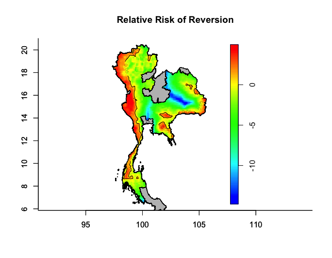
plot(imr_adapt_LINK, col = rev(rainbow(100, start = 0, end = 4/6)), main = "Relative Risk of Reversion")
plot(background, col = 'grey', add = T)
plot(imr_adapt_LINK, col = rev(rainbow(100, start = 0, end = 4/6)), add = T)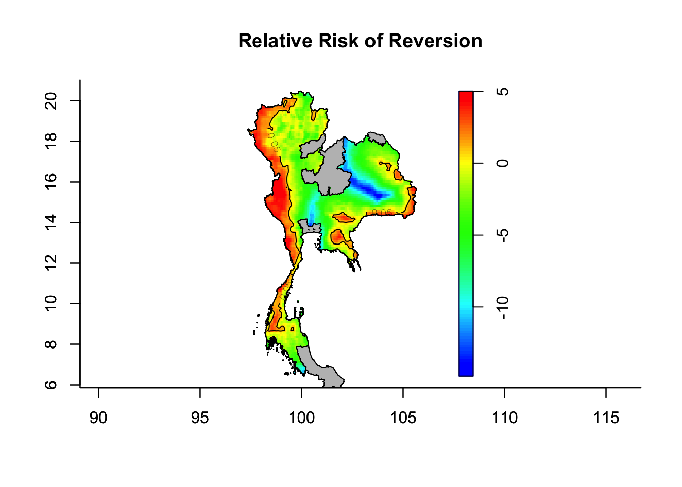
Interpretation
The relative risk map shows that the spatial intensity of foci that reverted is significantly higher than expected given the spatial intensity of non-active foci in areas along the eastern and western coasts that are known to have high local malaria transmission.
Force of Reversion
These results suggest that foci reversion is a non-random process in space and in terms of time-to-event (rate). In terms of transmission dynamics, the rate of reversion can be thought of as analogous to the force of infection (rate at which Susceptible (Non- active transmission foci) become Infected (Reverted foci)).
In transmission dynamics:
Force of Infection (lamda) = Contact rate (alpha) x Probability of transmission per contact (beta) x Proportion of the population that is infected
In our study alpha and beta were not measured directly, but their product can be estimated (for each district) by dividing the reversion rate by the proportion of active transmission foci per district. Overall, this equation shows how the Force of Reversion is primarily driven by the surrounding proportion of foci in which there is active transmission. Our model (not shown) and our relative risk map support this hypothesis as well.
Recommendations
Current guidelines do not require malaria prevention measures in non-active transmission foci that are located in high transmission districts. Although, sometimes prevention interventions are executed in these foci regardless. Our analysis suggests that these foci are at high risk of reversion due to both spatial intensity of reversion and transmission dynamic frameworks.
Therefore, we suggest that Thailand should consider expanding their interventions throughout districts with high proportion of active transmission foci.
)
Duncan Mahood
Epidemiology - Data Science
Duncan Mahood is an epidemiologist with Epidemiologic Research & Methods (ERM) with a focus on research for pharmaceutical and biotech clients.